
Copyright 2018 SIAM
In high school, I did research with the MIT PRIMES program. My project was to develop a faster and more accurate method of solving partial differential equations in two dimensions. In order to solve a PDE, the domain is broken into many smaller polygons (usually triangles or quadrilaterals) and the solution to the PDE is approximated with a piecewise polynomial. Finite element methods typically suffer from loss of precision when solving PDEs on meshes with skinny elements, and the computation time balloons when the polynomial approximant degree is increased. The method I developed is numerically stable on meshes with skinny elements. It is also significantly faster with higher polynomial degree approximants.
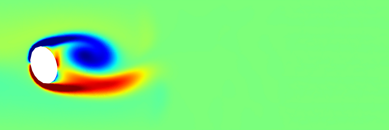
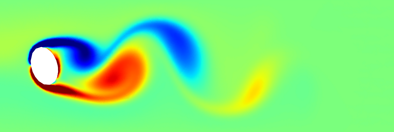
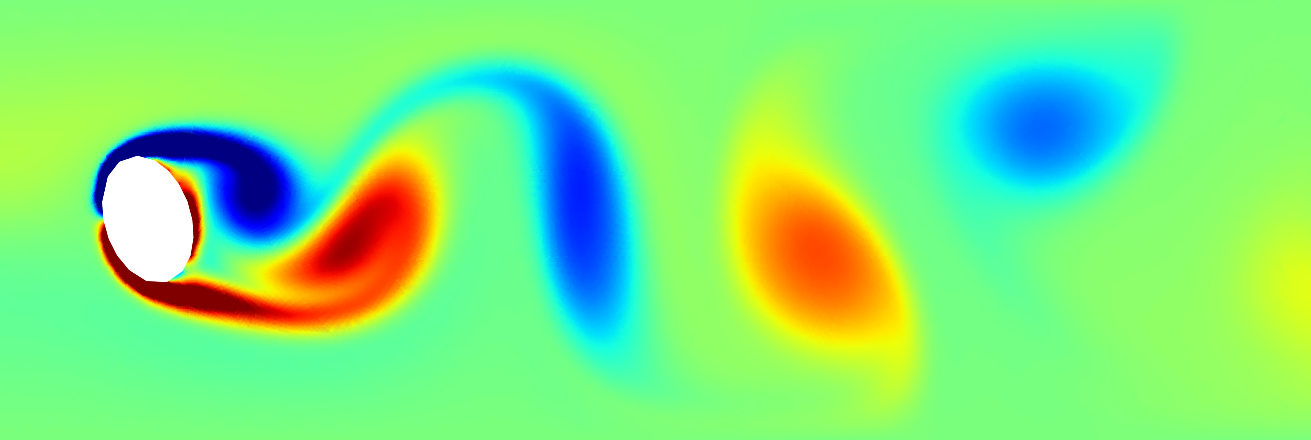
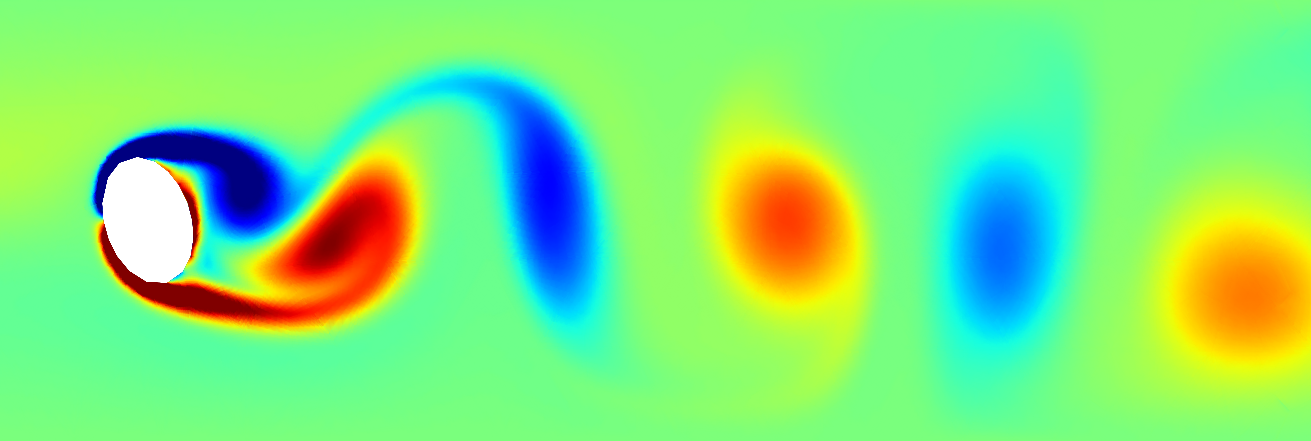
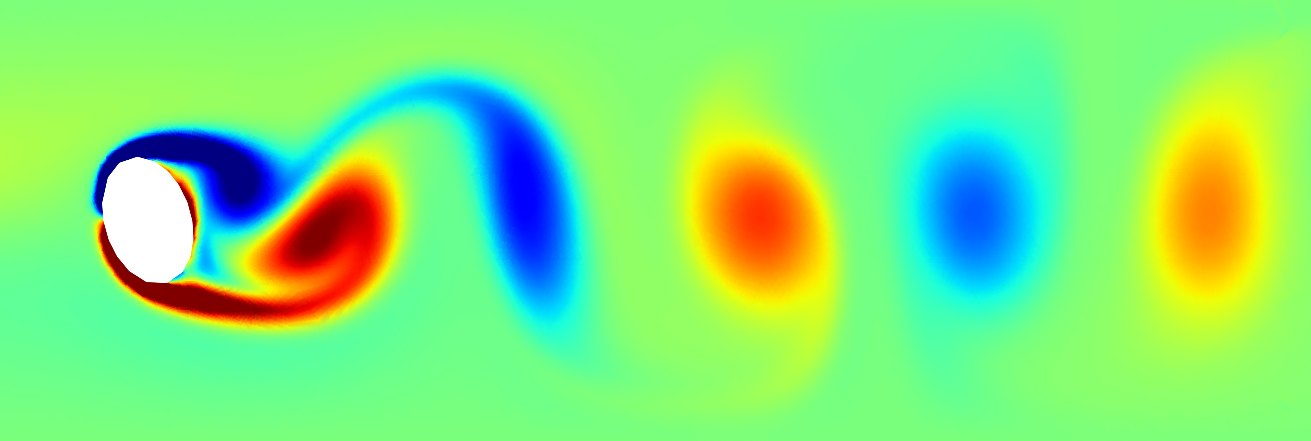
In order to test my method, I wrote a Navier-Stokes simulation. As I learned the hard way, the Navier-Stokes equations are a nightmare to simulate properly. There are a many different methods to choose from, all of which trade off accuracy, stability, computational complexity, and ease of implementation. Ultimately, I settled on a relatively simple explicit time stepping scheme for demonstration purposes, which suffered from questionable stability and required a very small time step.